Intruduction

Tabular Data-Processing Workflow

Titanic is perhaps the most familiar machine learning task for data scientists. The sub table after sampling is shown below:

Titanic Origin Data

Name	Age	SibSp	Ticket	Fare	Cabin	Embarked
Braund, Mr. Owen Harris	22	1	A/5 21171	7.25	NaN	S
Cumings, Mrs. John Bradley (Florence Briggs Thayer)	38	1	PC 17599	71.2833	C85	C
Heikkinen, Miss. Laina	26	0	STON/O2. 3101282	7.925	NaN	S
Futrelle, Mrs. Jacques Heath (Lily May Peel)	35	1	113803	53.1	C123	S
Allen, Mr. William Henry	35	0	373450	8.05	NaN	S
Moran, Mr. James	NaN	0	330877	8.4583	NaN	NaN
McCarthy, Mr. Timothy J	54	0	17463	51.8625	E46	S
Palsson, Master. Gosta Leonard	2	3	349909	21.075	NaN	S
Johnson, Mrs. Oscar W (Elisabeth Vilhelmina Berg)	27	0	347742	11.1333	NaN	S
Nasser, Mrs. Nicholas (Adele Achem)	14	1	237736	30.0708	NaN	C
Sandstrom, Miss. Marguerite Rut	4	1	PP 9549	16.7	G6	S
Bonnell, Miss. Elizabeth	58	0	113783	26.55	C103	S

You must notice that such raw table cannot be used in data-mining or machine-learning. We should fill the missing value, encoding the category value, and so on.

In order to introduce the practical problems this project wants to solve, I want to introduce a concept: feature group.

Feature Group

Except the columns that cannot provide entity specific properties, like id, the remaining columns are called features.

Note

You can find column_descriptions’s definition in autoflow.manager.data_manager.DataManager

If some features have similar properties, they are containing in a same feature group.

Note

You can find some feature group’s examples and practices in autoflow.hdl.hdl_constructor.HDL_Constructor

nan

nan is abbreviation of Not a Number, indicating that this column has missing value, like this:

>>> from numpy import NaN
>>> import pandas as pd
>>> import numpy as np
>>> column = [1, 2, 3, 4, NaN]

num

num is abbreviation of numerical, indicating that this column are all numerical value.

Note

Only num feature group can used in estimating phase

For example:

>>> column = [1, 2, 3, 4, 5]

cat

cat is abbreviation of categorical, indicating this column has any string-type value.

For example:

>>> column = [1, 2, 3, 4, "a"]

num_nan

num_nan is abbreviation of numerical NaN, indicating this column is full of numbers except for missing values.

For example:

>>> column = [1, 2, 3, 4, NaN]

cat_nan

cat_nan is abbreviation of categorical NaN, indicating this column has at least one string other than the missing value.

For example:

>>> column = [1, 2, 3, "a", NaN]

highR_nan

highR_nan is abbreviation of high ratio NaN, indicating this column has most of this column is missing.

For example:

>>> column = [1, 2, NaN, NaN, NaN]
>>> np.count_nonzero(pd.isna(column)) / column.size
0.6

NaN ratio is 0.6, more than 0.5 (default highR_nan_threshold)

lowR_nan

highR_nan is abbreviation of high ratio NaN, indicating this this column has most of this column is missing.

For example:

>>> column = [1, 2, 3, NaN, NaN]
>>> np.count_nonzero(pd.isna(column)) / column.size
0.4

NaN ratio is 0.4, less than 0.5 (default highR_nan_threshold)

highC_cat

highC_cat is abbreviation of high cardinality ratio categorical, indicating this this column is a categorical column (see in cat), and the unique value of this column divided by the total number of this column is more than highC_cat_threshold .

For example:

>>> column = ["a", "b", "c", "d", "d"]
>>> rows = len(column)
>>> np.unique(column).size / rows
0.8

cardinality ratio is 0.8, more than 0.5 (default highC_cat_threshold)

lowR_cat

lowR_cat is abbreviation of low cardinality ratio categorical, indicating this this column is a categorical column (see in cat), and the unique value of this column divided by the total number of this column is less than lowR_cat_threshold .

For example:

>>> column = ["a", "b", "d", "d", "d"]
>>> rows = len(column)
>>> np.unique(column).size / rows
0.4

cardinality ratio is 0.8, less than 0.5 (default lowR_cat_threshold)

Work Flow

After defining a concept: feature group, Workflow is the next important concept.

You can consider the whole machine-learning training and testing procedure as a directed acyclic graph(DAG), except ETL or other data prepare and feature extract procedure.

In this graph , you can consider nodes as feature group, edges as data-processing or estimating algorithms. Each edges’ tail node is a feature group before processing, each edges’ head node is a other feature group after processing.

You should keep in mind that, each edge represents one algorithm or a list of algorithms. For example, after a series of data-processing, single num (numerical) feature group is reserved, we should do estimating(fit features to target column):

In this figure we can see: lightgbm and random_forest are candidate algorithms. Some computer scientists said, AutoML is a CASH problem (Combined Algorithm Selection and Hyper-parameter optimization problem).

In fact, the algorithm selection on the edge allows this workflow to be called a workflow space.

Hear is the workflow space figure for Titanic task.

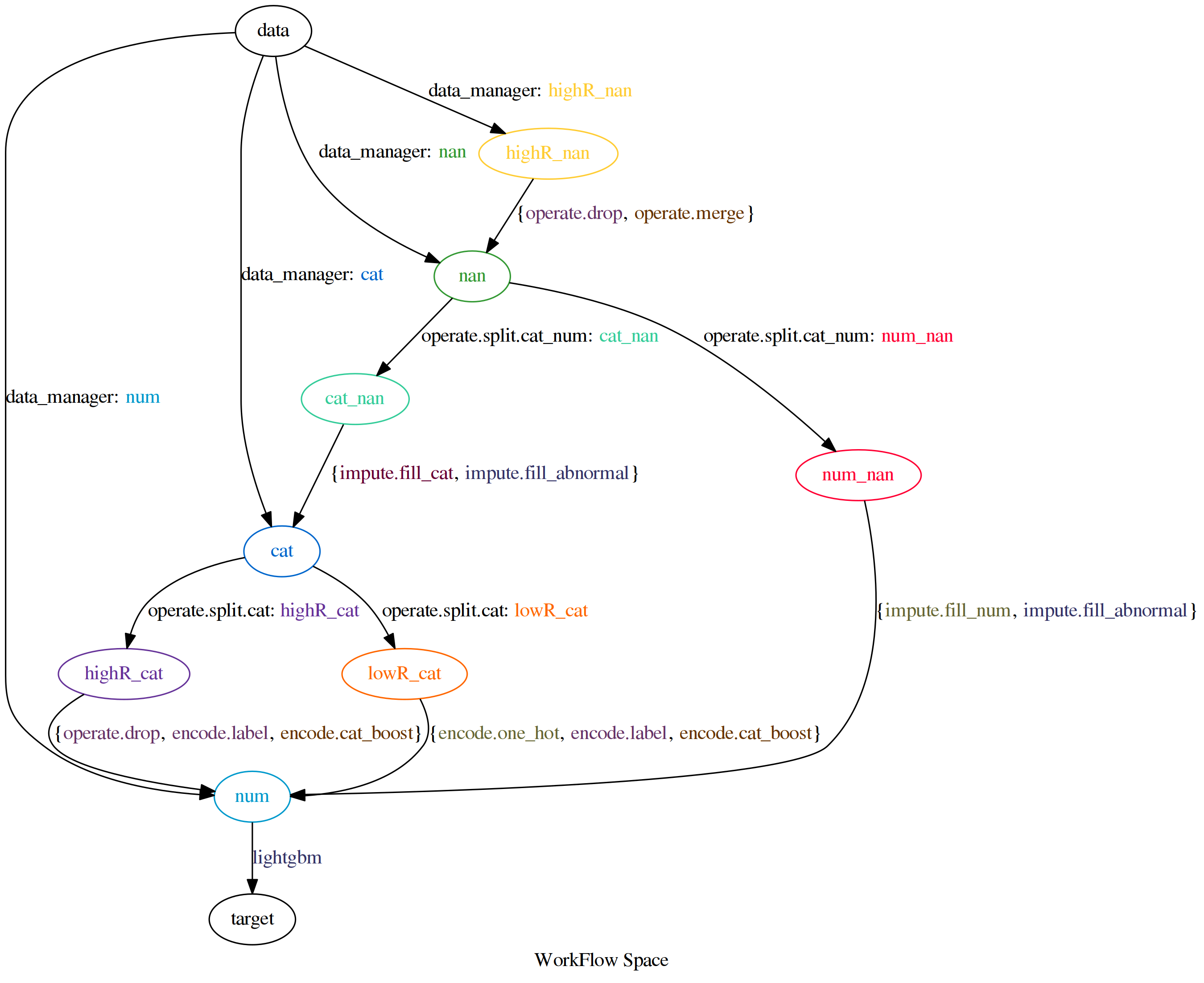
Instance In Titanic

You may be curious about the workflow space picture above, want to know how it work. Let me introduce the processing details step by step.

First step, data manager(autoflow.manager.data_manager.DataManager) split raw data into three feature group: nan, highR_nan, cat and num. like this:

First Step : Split By Data Manager

Name(cat)	Age(nan)	SibSp(num)	Ticket(cat)	Fare(num)	Cabin(highR_nan)	Embarked(nan)
Braund, Mr. Owen Harris	22	1	A/5 21171	7.25	NaN	S
Cumings, Mrs. John Bradley (Florence Briggs Thayer)	38	1	PC 17599	71.2833	C85	C
Heikkinen, Miss. Laina	26	0	STON/O2. 3101282	7.925	NaN	S
Futrelle, Mrs. Jacques Heath (Lily May Peel)	35	1	113803	53.1	C123	S
Allen, Mr. William Henry	35	0	373450	8.05	NaN	S
Moran, Mr. James	NaN	0	330877	8.4583	NaN	NaN
McCarthy, Mr. Timothy J	54	0	17463	51.8625	E46	S
Palsson, Master. Gosta Leonard	2	3	349909	21.075	NaN	S
Johnson, Mrs. Oscar W (Elisabeth Vilhelmina Berg)	27	0	347742	11.1333	NaN	S
Nasser, Mrs. Nicholas (Adele Achem)	14	1	237736	30.0708	NaN	C
Sandstrom, Miss. Marguerite Rut	4	1	PP 9549	16.7	G6	S
Bonnell, Miss. Elizabeth	58	0	113783	26.55	C103	S

This corresponds to this figure:

---

Second step, highR_nan_imputer should process highR_nan feature group to nan, merge (means don’t do any thing, just rename the feature group) and drop are candidate algorithms. in this case, we choose drop option.

Second Step : process highR nan

Name(cat)	Age(nan)	SibSp(num)	Ticket(cat)	Fare(num)	Embarked(nan)
Braund, Mr. Owen Harris	22	1	A/5 21171	7.25	S
Cumings, Mrs. John Bradley (Florence Briggs Thayer)	38	1	PC 17599	71.2833	C
Heikkinen, Miss. Laina	26	0	STON/O2. 3101282	7.925	S
Futrelle, Mrs. Jacques Heath (Lily May Peel)	35	1	113803	53.1	S
Allen, Mr. William Henry	35	0	373450	8.05	S
Moran, Mr. James	NaN	0	330877	8.4583	NaN
McCarthy, Mr. Timothy J	54	0	17463	51.8625	S
Palsson, Master. Gosta Leonard	2	3	349909	21.075	S
Johnson, Mrs. Oscar W (Elisabeth Vilhelmina Berg)	27	0	347742	11.1333	S
Nasser, Mrs. Nicholas (Adele Achem)	14	1	237736	30.0708	C
Sandstrom, Miss. Marguerite Rut	4	1	PP 9549	16.7	S
Bonnell, Miss. Elizabeth	58	0	113783	26.55	S

This corresponds to this figure:

---

Third step, using operate.split.cat_num algorithm to split nan to two feature groups: cat_nan and num_nan.

Third Step : Split Categorical and Numerical

Name(cat)	Age(num_nan)	SibSp(num_nan)	Ticket(cat)	Fare(num)	Embarked(cat_nan)
Braund, Mr. Owen Harris	22	1	A/5 21171	7.25	S
Cumings, Mrs. John Bradley (Florence Briggs Thayer)	38	1	PC 17599	71.2833	C
Heikkinen, Miss. Laina	26	0	STON/O2. 3101282	7.925	S
Futrelle, Mrs. Jacques Heath (Lily May Peel)	35	1	113803	53.1	S
Allen, Mr. William Henry	35	0	373450	8.05	S
Moran, Mr. James	NaN	0	330877	8.4583	NaN
McCarthy, Mr. Timothy J	54	0	17463	51.8625	S
Palsson, Master. Gosta Leonard	2	3	349909	21.075	S
Johnson, Mrs. Oscar W (Elisabeth Vilhelmina Berg)	27	0	347742	11.1333	S
Nasser, Mrs. Nicholas (Adele Achem)	14	1	237736	30.0708	C
Sandstrom, Miss. Marguerite Rut	4	1	PP 9549	16.7	S
Bonnell, Miss. Elizabeth	58	0	113783	26.55	S

This corresponds to this figure:

---

Fourth step, fill cat_nan to cat, fill num_nan to num.

Fourth Step : Fill NaN

Name(cat)	Age(num)	SibSp(num)	Ticket(cat)	Fare(num)	Embarked(cat)
Braund, Mr. Owen Harris	22	1	A/5 21171	7.25	S
Cumings, Mrs. John Bradley (Florence Briggs Thayer)	38	1	PC 17599	71.2833	C
Heikkinen, Miss. Laina	26	0	STON/O2. 3101282	7.925	S
Futrelle, Mrs. Jacques Heath (Lily May Peel)	35	1	113803	53.1	S
Allen, Mr. William Henry	35	0	373450	8.05	S
Moran, Mr. James	26.25	0	330877	8.4583	S
McCarthy, Mr. Timothy J	54	0	17463	51.8625	S
Palsson, Master. Gosta Leonard	2	3	349909	21.075	S
Johnson, Mrs. Oscar W (Elisabeth Vilhelmina Berg)	27	0	347742	11.1333	S
Nasser, Mrs. Nicholas (Adele Achem)	14	1	237736	30.0708	C
Sandstrom, Miss. Marguerite Rut	4	1	PP 9549	16.7	S
Bonnell, Miss. Elizabeth	58	0	113783	26.55	S

This corresponds to this figure:

---

Fifth step, using operate.split.cat algorithm to split cat to two feature groups: highC_cat and lowR_cat.

Fifth Step : Split Categorical to highC_cat and lowR_cat

Name(highC_cat)	Age(num)	SibSp(num)	Ticket(highC_cat)	Fare(num)	Embarked(lowR_cat)
Braund, Mr. Owen Harris	22	1	A/5 21171	7.25	S
Cumings, Mrs. John Bradley (Florence Briggs Thayer)	38	1	PC 17599	71.2833	C
Heikkinen, Miss. Laina	26	0	STON/O2. 3101282	7.925	S
Futrelle, Mrs. Jacques Heath (Lily May Peel)	35	1	113803	53.1	S
Allen, Mr. William Henry	35	0	373450	8.05	S
Moran, Mr. James	26.25	0	330877	8.4583	S
McCarthy, Mr. Timothy J	54	0	17463	51.8625	S
Palsson, Master. Gosta Leonard	2	3	349909	21.075	S
Johnson, Mrs. Oscar W (Elisabeth Vilhelmina Berg)	27	0	347742	11.1333	S
Nasser, Mrs. Nicholas (Adele Achem)	14	1	237736	30.0708	C
Sandstrom, Miss. Marguerite Rut	4	1	PP 9549	16.7	S
Bonnell, Miss. Elizabeth	58	0	113783	26.55	S

This corresponds to this figure:

---

Sixth step, we encode highC_cat to num by label_encoder, we encode lowR_cat to num by one_hot_encoder,

Sixth Step : Encoding Categorical to Numerical

Name(num)	Age(num)	SibSp(num)	Ticket(num)	Fare(num)	Embarked_1(num)	Embarked_2(num)
1	22	1	1	7.25	1	0
2	38	1	2	71.2833	0	1
3	26	0	3	7.925	1	0
4	35	1	4	53.1	1	0
5	35	0	5	8.05	1	0
6	26.25	0	6	8.4583	1	0
7	54	0	7	51.8625	1	0
8	2	3	8	21.075	1	0
9	27	0	9	11.1333	1	0
10	14	1	10	30.0708	0	1
11	4	1	11	16.7	1	0
12	58	0	12	26.55	0	1

This corresponds to this figure:

---

Seventh step, finally, we finish all the data preprocessing phase, now we should do estimating. lightgbm and random_forest are candidate algorithms.

This corresponds to this figure: