02. 多元变量

在本教程中，您将学习如何：

• 优化多元变量的目标函数

• 定义不同类型的搜索空间

优化多元变量的目标函数

# import fmin interface from UltraOpt
from ultraopt import fmin
# hdl2cs can convert HDL(Hyperparams Describe Language) to CS(Config Space)
from ultraopt.hdl import hdl2cs
import numpy as np
import pandas as pd
import seaborn as sns
from collections import Counter
%matplotlib inline

声明要优化的目标函数。与上次不同，我们将使用两个超参数\(x\)和\(y\)来优化函数。

\[z = sin\sqrt{x^2 + y^2}\]

def evaluate(config:dict):
    x, y = config['x'], config['y']
    return np.sin(np.sqrt(x**2 + y**2))

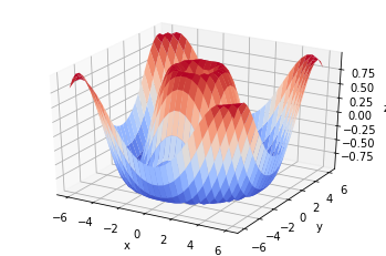
就像上次一样，我们尝试对其进行可视化。但与上次不同的是，这次有两个超参数，所以我们需要在三维空间中可视化它们。

import matplotlib.pyplot as plt
from matplotlib import cm
from mpl_toolkits.mplot3d import Axes3D

x = np.linspace(-6, 6, 30)
y = np.linspace(-6, 6, 30)
x, y = np.meshgrid(x, y)

z = evaluate({'x': x, 'y': y})

fig = plt.figure()
ax = plt.axes(projection='3d')
ax.plot_surface(x, y, z, cmap=cm.coolwarm)

ax.set_xlabel('x')
ax.set_ylabel('y')
ax.set_zlabel('z')

plt.show()

同样，让我们定义搜索空间。但这次，您需要定义两个超参数\((x,y)\)，因此将它们分别放在dict type 的 config 参数中。返回值 损失(loss) 越小， 配置(config) 越好。

重复 BasicTutorial 的步骤，让我们定义HDL \(\rightarrow\) 转为CS \(\rightarrow\) 采样config \(\rightarrow\) 评价config

HDL = {
    "x": {"_type": "uniform", "_value": [-6, 6]},
    "y": {"_type": "uniform", "_value": [-6, 6]},
}

CS = hdl2cs(HDL)
CS

Configuration space object:
  Hyperparameters:
    x, Type: UniformFloat, Range: [-6.0, 6.0], Default: 0.0
    y, Type: UniformFloat, Range: [-6.0, 6.0], Default: 0.0

configs = [config.get_dictionary() for config in CS.sample_configuration(5)]
configs

[{'x': 5.629597624120034, 'y': -3.8397274990916},
 {'x': 0.15448398644689476, 'y': 1.378628747372991},
 {'x': 4.807357592803779, 'y': 0.48761142925262746},
 {'x': 5.338999804636391, 'y': 1.8296410416479763},
 {'x': 0.6146223501865684, 'y': 0.5071135612795841}]

losses = [evaluate(config) for config in configs]
best_ix = np.argmin(losses)
print(f"optimal config: {configs[best_ix]}, \noptimal loss: {losses[best_ix]}")

optimal config: {'x': 4.807357592803779, 'y': 0.48761142925262746},
optimal loss: -0.9928523118019918

很好，让我们用UltraOpt来对评价函数进行优化吧！

result = fmin(
    eval_func=evaluate, # 评价函数
    config_space=HDL,   # 配置空间
    optimizer="ETPE", # 优化器
    n_iterations=100    #  迭代数
)

100%|██████████| 100/100 [00:00<00:00, 491.52trial/s, best loss: -1.000]

result

+---------------------------------+
| HyperParameters | Optimal Value |
+-----------------+---------------+
| x               | -2.5238       |
| y               | 3.9553        |
+-----------------+---------------+
| Optimal Loss    | -0.9998       |
+-----------------+---------------+
| Num Configs     | 100           |
+-----------------+---------------+

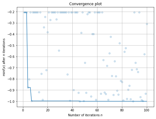
查看优化过程的拟合曲线：

plt.rcParams['figure.figsize'] = (8, 6)
result.plot_convergence();

定义不同类型的搜索空间

UltraOpt一共有8种类型的超参：

超参变量类型(_type)	参数列表(_value)	举例	描述
“choice”	options	["苹果","梨子","葡萄"]	选项(options)之间没有可比较关系
“ordinal”	sequence	["小学","中学","大学"]	序列(sequence)之间存在可比较关系
“uniform”	[low, high]	[0, 100]	均匀分布
“quniform”	[low, high, q]	[0, 100, 20]	间隔为 q 的离散均匀分布
“loguniform”	[low, high]	[0.1, 100]	log 缩放的均匀分布
“qloguniform”	[low, high, q]	[1, 100, 1]	log 缩放的离散均匀分布
“int_uniform”	[low, high]	[0, 10]	间隔为 1 的离散均匀分布， int类型
“int_quniform”	[low, high, q]	[0, 10, 2]	间隔为 q 的离散均匀分布， int类型

作为教学目的，我们定义一个空间，囊括所有类型的超参：

HDL = {
    "hp_choice": {"_type": "choice", "_value": ["apple", "pear", "grape"]},
    "hp_ordinal": {"_type": "ordinal", "_value": ["Primary school", "Middle school", "University"] },
    "hp_uniform": {"_type": "uniform", "_value": [0, 100]},
    "hp_quniform": {"_type": "quniform", "_value": [0, 100, 20]},
    "hp_loguniform": {"_type": "loguniform", "_value": [0.1, 100]},
    "hp_qloguniform": {"_type": "qloguniform", "_value": [10, 100, 10]},
    "hp_int_uniform": {"_type": "int_uniform", "_value": [0, 10]},
    "hp_int_quniform": {"_type": "int_quniform", "_value": [0, 10, 2]},
}

如果您定义的超参描述语言HDL可以正常被ultraopt.hdl.hdl2cs函数转换，说明您定义的HDL正确无误：

CS = hdl2cs(HDL)
CS

Configuration space object:
  Hyperparameters:
    hp_choice, Type: Categorical, Choices: {apple, pear, grape}, Default: apple
    hp_int_quniform, Type: UniformInteger, Range: [0, 10], Default: 5, Q: 2
    hp_int_uniform, Type: UniformInteger, Range: [0, 10], Default: 5
    hp_loguniform, Type: UniformFloat, Range: [0.1, 100.0], Default: 3.1622776602, on log-scale
    hp_ordinal, Type: Ordinal, Sequence: {Primary school, Middle school, University}, Default: Primary school
    hp_qloguniform, Type: UniformFloat, Range: [10.0, 100.0], Default: 31.6227766017, on log-scale, Q: 10.0
    hp_quniform, Type: UniformFloat, Range: [0.0, 100.0], Default: 50.0, Q: 20.0
    hp_uniform, Type: UniformFloat, Range: [0.0, 100.0], Default: 50.0

我们从配置空间CS中随机采样1000个：

configs = [config.get_dictionary() for config in CS.sample_configuration(1000)]
variables = {key:[config[key] for config in configs] for key in HDL}
hp_choice_cnt = Counter(variables["hp_choice"])
hp_ordinal_cnt = Counter(variables["hp_ordinal"])

然后可视化随机采样下各变量的分布：

plt.rcParams['figure.figsize'] = (20, 10); plt.subplot(2,4,1); plt.title("choice"); plt.pie(list(hp_choice_cnt.values()), labels=list(hp_choice_cnt.keys()), autopct='%1.0f%%');
plt.subplot(2,4,2); plt.title("ordinal"); plt.pie(list(hp_ordinal_cnt.values()), labels=list(hp_ordinal_cnt.keys()), autopct='%1.0f%%'); plt.subplot(2,4,3); plt.title("uniform"); sns.distplot(variables["hp_uniform"]); plt.subplot(2,4,4); plt.title("quniform"); plt.hist(variables["hp_quniform"], bins=20);
plt.subplot(2,4,5); plt.title("loguniform"); sns.distplot(variables["hp_loguniform"]); plt.subplot(2,4,6); plt.title("qloguniform"); plt.hist(variables["hp_qloguniform"], bins=25); plt.xticks(range(10,110,10));
plt.subplot(2,4,7); plt.title("int_uniform"); plt.xticks(range(11));plt.hist(variables["hp_int_uniform"], bins=30);plt.subplot(2,4,8); plt.title("int_quniform");plt.hist(variables["hp_int_quniform"], bins=20);

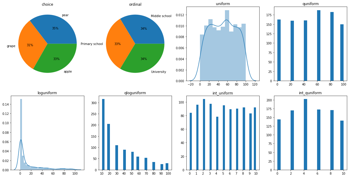
可以看到：

• 图1 图2 分别为 choice 选择类型超参 和 ordinal 有序类型超参。

  • 且他们都是离散变量。

  • 随机情况每个选项(option)被选中的几率都大约为 \(\frac{1}{3}\)。

• 图3 图5 分别是 uniform 和 loguniform。

  • 他们都是连续变量，所以用核密度估计图进行可视化。

  • uniform 类型的超参服从均匀分布。

  • loguniform 类型的超参在对其取对数后也服从均匀分布。

• 图4 的 quniform 间隔 q 为 10 。

• 图6 的 qloguniform 间隔 q 为 10 。

---

作为教学目的，我们定义一个依赖这8个变量的目标函数：

def evaluate(config: dict):
    choice2numerical = dict(zip(["apple", "pear", "grape"], [3,2,4]))
    ordinal2numerical = dict(zip(["Primary school", "Middle school", "University"], [1, 2, 3]))
    interact1 = np.sin(config["hp_int_uniform"] - choice2numerical[config["hp_choice"]]) * np.sin(config["hp_int_quniform"] - ordinal2numerical[config["hp_ordinal"]])
    interact2 = np.sin(config["hp_uniform"] - choice2numerical[config["hp_choice"]]*10) * np.sin(config["hp_quniform"] - ordinal2numerical[config["hp_ordinal"]]*10)
    interact3 = ((interact1 - np.log(config["hp_loguniform"])) - 2) ** 2 - ((interact2 - np.log(config["hp_qloguniform"])) - 1) ** 2
    return interact3

使用ultraopt.fmin进行优化：

result = fmin(
    eval_func=evaluate, # 评价函数
    config_space=HDL,   # 配置空间
    optimizer="ETPE", # 优化器
    n_iterations=200    #  迭代数
)

100%|██████████| 200/200 [00:04<00:00, 47.85trial/s, best loss: -43.363]

打印优化结果汇总表：

result

+---------------------------------+
| HyperParameters | Optimal Value |
+-----------------+---------------+
| hp_choice       | pear          |
| hp_int_quniform | 10            |
| hp_int_uniform  | 9             |
| hp_loguniform   | 0.2459        |
| hp_ordinal      | University    |
| hp_qloguniform  | 100.0000      |
| hp_quniform     | 0.0000        |
| hp_uniform      | 100.0000      |
+-----------------+---------------+
| Optimal Loss    | -43.3633      |
+-----------------+---------------+
| Num Configs     | 200           |
+-----------------+---------------+

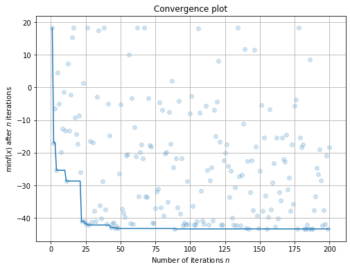
查看优化过程的拟合曲线：

plt.rcParams['figure.figsize'] = (8, 6)
result.plot_convergence();