05. 实现一个简单的AutoML系统¶

AutoML系统的顶层设计¶

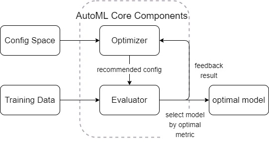
我们在上个教程中，学习到了UltraOpt的设计哲学是将优化器与评价器分离，如图所示:

[1]:

from graphviz import Digraph; g = Digraph()
g.node("config space", shape="ellipse"); g.node("optimizer", shape="box")
g.node("config", shape="ellipse"); g.node("loss", shape="circle"); g.node("evaluator", shape="box")
g.edge("config space", "optimizer", label="initialize"); g.edge("optimizer", "config", label="<<b>ask</b>>", color='blue')
g.edge("config","evaluator" , label="send to"); g.edge("evaluator","loss" , label="evaluate")
g.edge("config", "optimizer", label="<<b>tell</b>>", color='red'); g.edge("loss", "optimizer", label="<<b>tell</b>>", color='red')
g.graph_attr['rankdir'] = 'LR'; g

[1]:

../_images/_tutorials_05._Implement_a_Simple_AutoML_System_3_0.svg

而当我们要解决AutoML问题时，我们可以这样定义AutoML系统结构：

用HDL定义一个简单的AutoML配置空间¶

在03. Conditional Parameter教程中，我们知道了AutoML问题的优化可以视为一个CASH问题，不仅涉及算法选择，还涉及超参优化。我们用HDL定义一个简单的CASH问题的配置空间：

[2]:

from ultraopt.hdl import hdl2cs, plot_hdl, layering_config, plot_layered_dict
HDL = {
    'classifier(choice)':{
        "LinearSVC": {
          "max_iter": {"_type": "int_quniform","_value": [300, 3000, 100], "_default": 600},
          "penalty":  {"_type": "choice", "_value": ["l1", "l2"],"_default": "l2"},
          "dual": {"_type": "choice", "_value": [True, False],"_default": False},
          "loss":  {"_type": "choice", "_value": ["hinge", "squared_hinge"],"_default": "squared_hinge"},
          "C": {"_type": "loguniform", "_value": [0.01, 10000],"_default": 1.0},
          "multi_class": "ovr",
          "random_state": 42,
          "__forbidden": [
              {"penalty": "l1","loss": "hinge"},
              {"penalty": "l2","dual": False,"loss": "hinge"},
              {"penalty": "l1","dual": False},
              {"penalty": "l1","dual": True,"loss": "squared_hinge"},
          ]
        },
        "RandomForestClassifier": {
          "n_estimators": {"_type": "int_quniform","_value": [10, 200, 10], "_default": 100},
          "criterion": {"_type": "choice","_value": ["gini", "entropy"],"_default": "gini"},
          "max_features": {"_type": "choice","_value": ["sqrt","log2"],"_default": "sqrt"},
          "min_samples_split": {"_type": "int_uniform", "_value": [2, 20],"_default": 2},
          "min_samples_leaf": {"_type": "int_uniform", "_value": [1, 20],"_default": 1},
          "bootstrap": {"_type": "choice","_value": [True, False],"_default": True},
          "random_state": 42
        },
        "KNeighborsClassifier": {
          "n_neighbors": {"_type": "int_loguniform", "_value": [1,100],"_default": 3},
          "weights" : {"_type": "choice", "_value": ["uniform", "distance"],"_default": "uniform"},
          "p": {"_type": "choice", "_value": [1, 2],"_default": 2},
        },
    }
}

[3]:

CS = hdl2cs(HDL)
g = plot_hdl(HDL)
g.graph_attr['size'] = "15,8"
g

[3]:

../_images/_tutorials_05._Implement_a_Simple_AutoML_System_9_0.svg

定义一个简单的AutoML评价器¶

在定义好了配置空间之后，现在我们来看评价器。

在UltraOpt的设计哲学中，评价器可以是一个类（实现__call__魔法方法），也可以是个函数。但其必须满足：

接受 dict 类型参数 config
返回 float 类型参数 loss

在AutoML问题中，评价器的工作流程如下： 1. 将config转化为一个机器学习模型 2. 在训练集上对机器学习模型进行训练 3. 在验证集上得到相应的评价指标 4. 对评价指标进行处理，使其越小越好，返回loss

在了解了这些知识后，我们来开发 AutoML 评价器

为了方便同学们理解，我们先顺序地将之前提到的AutoML 评价器工作流程跑一遍：

Step 1. 将config转化为一个机器学习模型¶

[4]:

# 引入 sklearn 的分类器
from sklearn.svm import LinearSVC
from sklearn.ensemble import RandomForestClassifier
from sklearn.neighbors import KNeighborsClassifier

假设评价器传入了一个 config 参数，我们先通过获取配置空间默认值（也可以对配置空间 CS 对象进行采样）得到 config

[5]:

config = CS.get_default_configuration().get_dictionary()
config

[5]:

{'classifier:__choice__': 'LinearSVC',
 'classifier:LinearSVC:C': 1.0,
 'classifier:LinearSVC:dual': 'True:bool',
 'classifier:LinearSVC:loss': 'squared_hinge',
 'classifier:LinearSVC:max_iter': 600,
 'classifier:LinearSVC:multi_class': 'ovr',
 'classifier:LinearSVC:penalty': 'l2',
 'classifier:LinearSVC:random_state': '42:int'}

我们用配置分层函数 ultraopt.hdl.layering_config 处理这个配置

[6]:

layered_dict = layering_config(config)
layered_dict

[6]:

{'classifier': {'LinearSVC': {'C': 1.0,
   'dual': True,
   'loss': 'squared_hinge',
   'max_iter': 600,
   'multi_class': 'ovr',
   'penalty': 'l2',
   'random_state': 42}}}

[8]:

plot_layered_dict(layered_dict)

[8]:

../_images/_tutorials_05._Implement_a_Simple_AutoML_System_18_0.svg

我们需要获取这个配置的如下信息：

算法选择的结果
被选择算法对应的参数

[9]:

AS_HP = layered_dict['classifier'].copy()
AS, HP = AS_HP.popitem()
AS  # 算法选择的结果

[9]:

'LinearSVC'

[10]:

HP  # 被选择算法对应的参数

[10]:

{'C': 1.0,
 'dual': True,
 'loss': 'squared_hinge',
 'max_iter': 600,
 'multi_class': 'ovr',
 'penalty': 'l2',
 'random_state': 42}

根据 算法选择结果 + 对应的参数 实例化一个 机器学习对象

[11]:

ML_model = eval(AS)(**HP)
ML_model # 实例化的机器学习对象

[11]:

LinearSVC(C=1.0, class_weight=None, dual=True, fit_intercept=True,
          intercept_scaling=1, loss='squared_hinge', max_iter=600,
          multi_class='ovr', penalty='l2', random_state=42, tol=0.0001,
          verbose=0)

Step 2. 在训练集上对机器学习模型进行训练¶

我们采用MNIST手写数字数据集的一个子集来作为训练数据：

[12]:

from sklearn.datasets import load_digits
import seaborn as sns
import warnings
warnings.filterwarnings("ignore")
X, y = load_digits(return_X_y=True)

[13]:

digit = X[0].reshape([8, 8])
sns.heatmap(digit, annot=True);

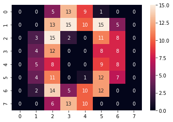
../_images/_tutorials_05._Implement_a_Simple_AutoML_System_27_0.png

[14]:

y[0]

[14]:

我们需要划分一个训练集与验证集，在训练集上训练 Step 1得到的机器学习模型，在验证集上预测，预测值会被处理为返回的损失值 loss 。首先我们要对原数据进行切分以得到训练集和验证集：

[15]:

from sklearn.model_selection import train_test_split

[16]:

X_train, X_test, y_train, y_test = train_test_split(
     X, y, test_size=0.33, random_state=42)

然后我们需要在训练集X_train，y_train上对机器学习模型ML_model进行训练：

[17]:

ML_model.fit(X_train, y_train)

[17]:

LinearSVC(C=1.0, class_weight=None, dual=True, fit_intercept=True,
          intercept_scaling=1, loss='squared_hinge', max_iter=600,
          multi_class='ovr', penalty='l2', random_state=42, tol=0.0001,
          verbose=0)

Step 3. 在验证集上得到相应的评价指标¶

为了保证我们的机器学习模型具有对未知数据的泛化能力，所以需要用未参与训练的验证集来评价之前得到的机器学习模型。

所以，我们需要一个评价指标。这里我们选用最简单的 accuracy_score

[18]:

from sklearn.metrics import accuracy_score

[19]:

y_pred = ML_model.predict(X_test)

[20]:

accuracy = accuracy_score(y_test, y_pred)
accuracy

[20]:

0.9444444444444444

我们注意到本示例的 Step 2与Step 3的训练与验证部分可能存在偏差。比如如果数据集划分得不均匀，可能会在验证集上过拟合。

我们可以用交叉验证(Cross Validation, CV)的方法解决这个问题，交叉验证的原理如图所示：

e4ecbba2a4b04906814183e51d1ecd9a

[21]:

from sklearn.model_selection import StratifiedKFold # 采用分层抽样
from sklearn.model_selection import cross_val_score

因为这只是一个简单的示例，所以采用3-Folds交叉验证以减少计算时间。

在实践中建议使用5-Folds交叉验证或10-Folds交叉验证。

[22]:

cv = StratifiedKFold(n_splits=3, shuffle=True, random_state=0)

[23]:

scores = cross_val_score(ML_model, X, y, cv=cv)
scores

[23]:

array([0.92654424, 0.94490818, 0.96327212])

我们采用交叉验证的平均值作为最后的得分：

[24]:

score = scores.mean()
score

[24]:

0.9449081803005009

Step 4. 对评价指标进行处理，使其越小越好，返回loss¶

我们注意到，评价指标正确率的取值范围是0-1，且是越大越好的，所以我们需要将score处理为越小越好的loss：

[25]:

loss = 1 - score
loss

[25]:

0.055091819699499056

用一个函数实现AutoML评价器¶

[26]:

metric = "accuracy"
def evaluate(config: dict) -> float:
    layered_dict = layering_config(config)
    display(plot_layered_dict(layered_dict))  # 用于在jupyter notebook中可视化，实践中可以删除次行
    AS_HP = layered_dict['classifier'].copy()
    AS, HP = AS_HP.popitem()
    ML_model = eval(AS)(**HP)
    # 注意到： X, y, cv, metric 都是函数外的变量
    scores = cross_val_score(ML_model, X, y, cv=cv, scoring=metric)
    score = scores.mean()
    print(f"accuracy: {score:}") # 用于在jupyter notebook中调试，实践中可以删除次行
    return 1 - score

[27]:

evaluate(CS.get_default_configuration())

../_images/_tutorials_05._Implement_a_Simple_AutoML_System_52_0.svg

accuracy: 0.9449081803005009

[27]:

0.055091819699499056

用一个类实现AutoML评价器¶

我们注意到，evaluate函数的 X, y, cv, metric 都是函数外的变量，不利于管理，所以实践中我们一般采用定义类来实现评价器。

首先我们定义一个类，这个类需要根据训练数据、评价指标和交叉验证方法等条件进行初始化：

[28]:

default_cv = StratifiedKFold(n_splits=3, shuffle=True, random_state=0)

class Evaluator():
    def __init__(self,
        X, y,
        metric="accuracy",
        cv=default_cv):
        # 初始化
        self.X = X
        self.y = y
        self.metric = metric
        self.cv = cv

然后我们需要实现__call__魔法方法，在该方法中实现整个评价过程：

[29]:

default_cv = StratifiedKFold(n_splits=3, shuffle=True, random_state=0)

class Evaluator():
    def __init__(self,
        X, y,
        metric="accuracy",
        cv=default_cv):
        # 初始化
        self.X = X
        self.y = y
        self.metric = metric
        self.cv = cv

    def __call__(self, config: dict) -> float:
        layered_dict = layering_config(config)
        AS_HP = layered_dict['classifier'].copy()
        AS, HP = AS_HP.popitem()
        ML_model = eval(AS)(**HP)
        scores = cross_val_score(ML_model, self.X, self.y, cv=self.cv, scoring=self.metric)
        score = scores.mean()
        return 1 - score

实例化一个评价器对象：

[30]:

evaluator = Evaluator(X, y)

用配置空间的一个采样样本测试这个AutoML评价器：

[31]:

evaluator(CS.sample_configuration())

[31]:

0.017250973845297835

根据上述知识实现一个简单的AutoML系统¶

配置空间 、评价器我们都有了，UltraOpt已经实现了成熟的优化器，所以我们只需要用ultraopt.fmin函数将这些组件串起来

[32]:

from ultraopt import fmin

[33]:

result = fmin(evaluator, HDL, optimizer="ETPE", n_iterations=40)
result

100%|██████████| 40/40 [00:14<00:00,  2.67trial/s, best loss: 0.012]

[33]:

+----------------------------------------------------------------------------+
| HyperParameters                                     | Optimal Value        |
+-----------------------------------------------------+----------------------+
| classifier:__choice__                               | KNeighborsClassifier |
| classifier:KNeighborsClassifier:n_neighbors         | 4                    |
| classifier:KNeighborsClassifier:p                   | 2:int                |
| classifier:KNeighborsClassifier:weights             | distance             |
| classifier:LinearSVC:C                              | -                    |
| classifier:LinearSVC:dual                           | -                    |
| classifier:LinearSVC:loss                           | -                    |
| classifier:LinearSVC:max_iter                       | -                    |
| classifier:LinearSVC:multi_class                    | -                    |
| classifier:LinearSVC:penalty                        | -                    |
| classifier:LinearSVC:random_state                   | -                    |
| classifier:RandomForestClassifier:bootstrap         | -                    |
| classifier:RandomForestClassifier:criterion         | -                    |
| classifier:RandomForestClassifier:max_features      | -                    |
| classifier:RandomForestClassifier:min_samples_leaf  | -                    |
| classifier:RandomForestClassifier:min_samples_split | -                    |
| classifier:RandomForestClassifier:n_estimators      | -                    |
| classifier:RandomForestClassifier:random_state      | -                    |
+-----------------------------------------------------+----------------------+
| Optimal Loss                                        | 0.0117               |
+-----------------------------------------------------+----------------------+
| Num Configs                                         | 40                   |
+-----------------------------------------------------+----------------------+

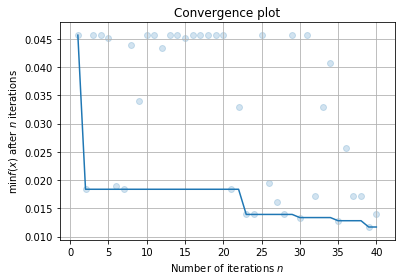
我们可以对AutoML得到的结果进行数据分析：

首先，我们可以绘制拟合曲线：

[34]:

result.plot_convergence();

../_images/_tutorials_05._Implement_a_Simple_AutoML_System_68_0.png

然后，我们想用hiplot绘制高维交互图。我们先整理出数据：

[35]:

data = result.plot_hi(return_data_only=True, target_name="accuracy", loss2target_func=lambda loss: 1 - loss)

如果直接绘图的话，您会发现由于算法选择的存在，会导致高维交互图非常的杂乱。我们简单编写一个函数，对不同的算法选择结果的超参进行可视化：

[36]:

import hiplot as hip

[37]:

def viz_subset(model_name, data):
    data_filtered = []
    for datum  in data:
        if datum["classifier:__choice__"] == model_name:
            datum = datum.copy()
            score = datum.pop("accuracy")
            AS, HP = layering_config(datum)["classifier"].popitem()
            HP["accuracy"]  = score
            data_filtered.append(HP)
    hip.Experiment.from_iterable(data_filtered).display()

我们简单地对随机森林 RandomForestClassifier 进行可视化：

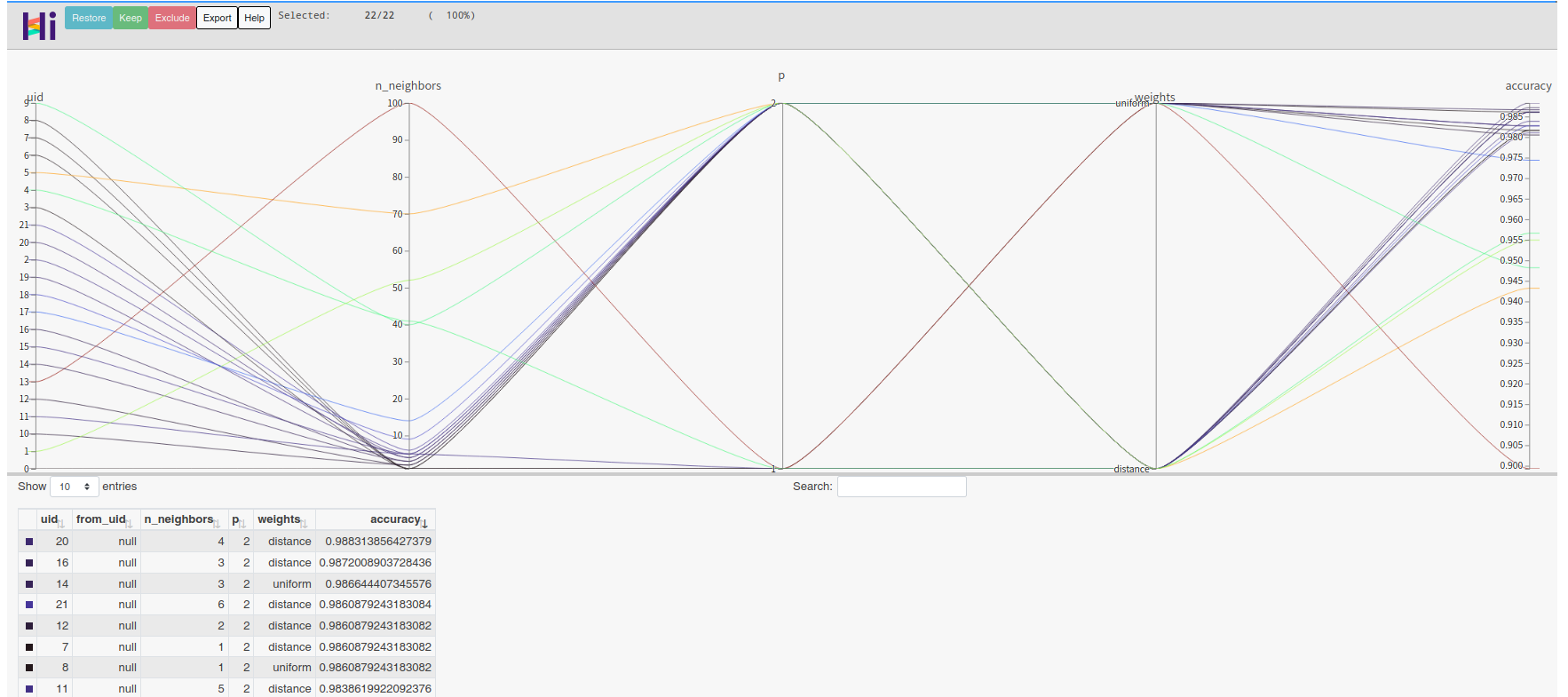
因为绘制hiplot高维交互图后jupyter notebook的文件大小会大量增加，所以我们以截图代替。您可以在自己的notebook中取消注释并执行以下代码：

[40]:

#viz_subset("RandomForestClassifier", data)

[42]:

#viz_subset("LinearSVC", data)

[42]:

#viz_subset("KNeighborsClassifier", data)

我们将所有代码整理为了 05. Implement a Simple AutoML System.py 脚本。

您可以在这个脚本中更直接地学习一个简单AutoML系统的搭建方法。