06. 结合多保真优化
多保真优化简介
在上一个教程中,我们学习了如何实现一个简单的AutoML系统。但这个AutoML系统的核心:贝叶斯优化算法往往需要大量对采样的评价才能获得比较好的结果。
然而,在自动机器学习(Automatic Machine Learning, AutoML)任务中评价往往通过 k 折交叉验证获得,在大数据集的机器学习任务上,获得一个评价的时间代价巨大。这也影响了优化算法在自动机器学习问题上的效果。所以一些减少评价代价的方法被提出来,其中多保真度优化(Multi-Fidelity Optimization)[1]就是其中的一种。而多臂老虎机算法(Multi-armed Bandit Algorithm,
MBA)[2]是多保真度算法的一种。在此基础上,有两种主流的bandit-based优化策略:
首先我们介绍连续减半(Successive Halving ,SH)。在连续减半策略中, 我们将评价代价参数化为一个变量budget,即预算。根据BOHB论文[5]的阐述,我们可以根据不同的场景定义不同的budget,举例如下:
迭代算法的迭代数(如:神经网络的epoch、随机森林,GBDT的树的个数)
机器学习算法所使用的样本数
贝叶斯神经网络[6]中MCMC链的长度
深度强化学习中的尝试数
举例说明,我们定义\(budget_{max}=1\), \(budget_{min}=\frac{1}{8}\), \(\eta=2\) (eta = 2) 。在这里budget的语义表示使用\(100\times budget\)%的样本。
首先我们从配置空间(或称为超参空间)随机采样8个配置,实例化为8个机器学习模型。
然后用\(\frac{1}{8}\)的训练样本训练这8个模型并在验证集得到相应的损失值。
保留这8个模型中loss最低的前4个模型,其余的舍弃。
依次类推,最后仅保留一个模型,并且其
budget=1(可以用全部的样本进行训练)
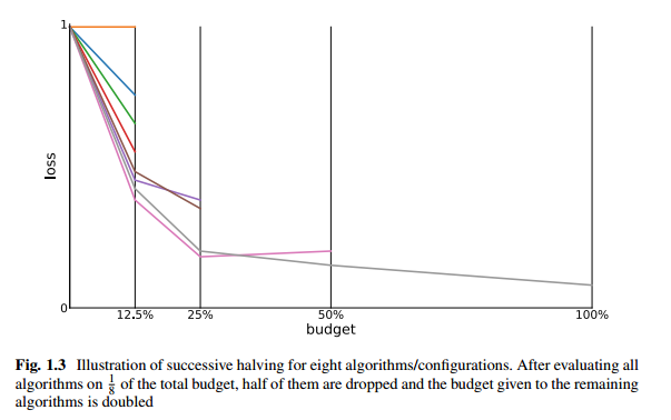
上图描述了例子中的迭代过程(图片来自[1]) 。我们可以用ultraopt.multi_fidelity中的SuccessiveHalvingIterGenerator来实例化这一过程:
[1]:
from ultraopt.multi_fidelity import SuccessiveHalvingIterGenerator, HyperBandIterGenerator
[2]:
SH = SuccessiveHalvingIterGenerator(min_budget=1/8, max_budget=1, eta=2)
SH.get_table()
[2]:
| iter 0 | ||||
|---|---|---|---|---|
| stage 0 | stage 1 | stage 2 | stage 3 | |
| num_config | 8 | 4 | 2 | 1 |
| budget | 1/8 | 1/4 | 1/2 | 1 |
接下来我们介绍HyperBand(HB)的策略。
[3]:
SH = HyperBandIterGenerator(min_budget=1/8, max_budget=1, eta=2)
SH.get_table()
[3]:
| iter 0 | iter 1 | iter 2 | iter 3 | |||||||
|---|---|---|---|---|---|---|---|---|---|---|
| stage 0 | stage 1 | stage 2 | stage 3 | stage 0 | stage 1 | stage 2 | stage 0 | stage 1 | stage 0 | |
| num_config | 8 | 4 | 2 | 1 | 4 | 2 | 1 | 4 | 2 | 4 |
| budget | 1/8 | 1/4 | 1/2 | 1 | 1/4 | 1/2 | 1 | 1/2 | 1 | 1 |
在UltraOpt中结合贝叶斯优化与多保真优化
我们注意到,上文描述的SH和HB策略在采样时都是随机采样,而UltraOpt将优化器和多保真迭代生成器这两个部分解耦和了,您可以将任意的贝叶斯优化算法和多保真优化算法进行组合。
这样的组合其实就是BOHB(Bayesian Optimization Hyperband)算法[5]。UltraOpt在很多代码上借鉴和直接使用了HpBandSter[7]这个开源项目,我们感谢他们优秀的工作。
如果您需要采用多保真优化策略,您的评价函数需要增加一个float类型的budget参数:
def evaluate(config: dict, budget:float) -> float :
    pass
为了测试, 我们采用ultraopt.tests.mock中自带的一个含有budget的评价函数,以及相应的配置空间:
[4]:
from ultraopt.tests.mock import evaluate, config_space
from ultraopt import fmin
from ultraopt.multi_fidelity import HyperBandIterGenerator
在调用ultraopt.fmin函数时,采用多保真策略时需要做以下修改:
需要指定
multi_fidelity_iter_generator(多保真迭代生成器)n_iterations参数与普通模式不同,不再代表评价函数的调用次数,而代表iter_generator的迭代次数,需要酌情设置parallel_strategy需要设置为AsyncComm,不改变默认值就没事
首先我们实例化一个iter_generator(多保真迭代生成器),并根据get_table()函数的可视化结果设置n_iterations。
因为测试函数的max_budget = 100, 我们按照25, 50, 100来递增budget:
[5]:
iter_generator = HyperBandIterGenerator(min_budget=25, max_budget=100, eta=2)
iter_generator.get_table()
[5]:
| iter 0 | iter 1 | iter 2 | ||||
|---|---|---|---|---|---|---|
| stage 0 | stage 1 | stage 2 | stage 0 | stage 1 | stage 0 | |
| num_config | 4 | 2 | 1 | 2 | 1 | 3 |
| budget | 25 | 50 | 100 | 50 | 100 | 100 |
[6]:
result = fmin(evaluate, config_space, n_iterations=50, multi_fidelity_iter_generator=iter_generator, n_jobs=3)
result
100%|██████████| 218/218 [00:00<00:00, 247.44trial/s, max budget: 100.0, best loss: 0.540]
[6]:
+------------------------------------------------------+
| HyperParameters | Optimal Value                      |
+-----------------+---------------+--------+-----------+
| x0              | 0.1594        | 0.0317 | 0.2921    |
| x1              | 3.3435        | 1.8980 | 0.0657    |
+-----------------+---------------+--------+-----------+
| Budgets         | 25            | 50     | 100 (max) |
+-----------------+---------------+--------+-----------+
| Optimal Loss    | 5.6924        | 4.0304 | 0.5397    |
+-----------------+---------------+--------+-----------+
| Num Configs     | 68            | 68     | 82        |
+-----------------+---------------+--------+-----------+
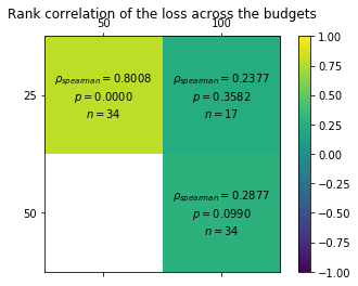
按budget分组的随时间变化拟合曲线:
[7]:
result.plot_convergence_over_time(yscale="log");
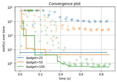
low_budget推荐得到的优势配置会保留到high_budget,从而可以根据loss-pairs计算不同budget之间的相关性:
[8]:
result.plot_correlation_across_budgets();
AutoML场景下的多保真优化
虽然ultraopt.tests.mock中提供的合成函数可以测试结合多保真策略的优化,但这毕竟不是真实场景。
现在,我们就通过修改教程05. Implement a Simple AutoML System中的AutoML评价器,将其改造为一个支持多保真优化的评价器,并进行相应的测试。
[9]:
from sklearn.svm import LinearSVC
from sklearn.ensemble import RandomForestClassifier
from sklearn.neighbors import KNeighborsClassifier
from sklearn.datasets import load_digits
import seaborn as sns
import numpy as np
import warnings
from ultraopt.hdl import layering_config
from sklearn.model_selection import StratifiedKFold # 采用分层抽样

warnings.filterwarnings("ignore")
X, y = load_digits(return_X_y=True)
cv = StratifiedKFold(n_splits=3, shuffle=True, random_state=0)

def evaluate(config: dict, budget: float) -> float:
    layered_dict = layering_config(config)
    AS_HP = layered_dict['classifier'].copy()
    AS, HP = AS_HP.popitem()
    ML_model = eval(AS)(**HP)
    # 注释掉采用原版的采用所有数据进行训练的方法(相当于budget=1)
    # scores = cross_val_score(ML_model, X, y, cv=cv, scoring=metric)
    # -------------------------------------------------------------
    # 采用在对【 5折交叉验证中的训练集 】进行采样的方法,采样率为 budget
    sample_ratio  = budget
    scores = []
    for i, (train_ix, valid_ix) in enumerate(cv.split(X, y)):
        rng = np.random.RandomState(i)
        size = int(train_ix.size * sample_ratio)
        train_ix = rng.choice(train_ix, size, replace=False)
        X_train = X[train_ix, :]
        y_train = y[train_ix]
        X_valid = X[valid_ix, :]
        y_valid = y[valid_ix]
        ML_model.fit(X_train, y_train)
        scores.append(ML_model.score(X_valid, y_valid))
    # -------------------------------------------------------------
    score = np.mean(scores)
    return 1 - score
[10]:
config = {'classifier:__choice__': 'LinearSVC',
 'classifier:LinearSVC:C': 1.0,
 'classifier:LinearSVC:dual': 'True:bool',
 'classifier:LinearSVC:loss': 'squared_hinge',
 'classifier:LinearSVC:max_iter': 600,
 'classifier:LinearSVC:multi_class': 'ovr',
 'classifier:LinearSVC:penalty': 'l2',
 'classifier:LinearSVC:random_state': '42:int'}
[11]:
evaluate(config, 0.125)
[11]:
0.12298274902615469
[12]:
evaluate(config, 0.5)
[12]:
0.0690038953811909
[13]:
evaluate(config, 1)
[13]:
0.05286588759042843
可以看到我们已经成功定义了一个结合多保真策略的AutoML评价器,并且按照一般规律:budget越大,评价代价也越大,模型表现也越好,loss越小。
我们将上述代码整合到05. Implement a Simple AutoML System.py脚本中,形成06. Combine Multi-Fidelity Optimization.py脚本:
[14]:
#!/usr/bin/env python
# -*- coding: utf-8 -*-
# @Author  : qichun tang
# @Date    : 2020-12-28
# @Contact    : qichun.tang@bupt.edu.cn
import warnings

from sklearn.svm import LinearSVC
from sklearn.ensemble import RandomForestClassifier
from sklearn.neighbors import KNeighborsClassifier
from sklearn.datasets import load_digits
from sklearn.model_selection import StratifiedKFold  # 采用分层抽样
from sklearn.model_selection import cross_val_score
import sklearn.metrics
import numpy as np

from ultraopt import fmin
from ultraopt.hdl import hdl2cs, plot_hdl, layering_config
from ultraopt.multi_fidelity import HyperBandIterGenerator

warnings.filterwarnings("ignore")
HDL = {
    'classifier(choice)':{
        "LinearSVC": {
          "max_iter": {"_type": "int_quniform","_value": [300, 3000, 100], "_default": 600},
          "penalty":  {"_type": "choice", "_value": ["l1", "l2"],"_default": "l2"},
          "dual": {"_type": "choice", "_value": [True, False],"_default": False},
          "loss":  {"_type": "choice", "_value": ["hinge", "squared_hinge"],"_default": "squared_hinge"},
          "C": {"_type": "loguniform", "_value": [0.01, 10000],"_default": 1.0},
          "multi_class": "ovr",
          "random_state": 42,
          "__forbidden": [
              {"penalty": "l1","loss": "hinge"},
              {"penalty": "l2","dual": False,"loss": "hinge"},
              {"penalty": "l1","dual": False},
              {"penalty": "l1","dual": True,"loss": "squared_hinge"},
          ]
        },
        "RandomForestClassifier": {
          "n_estimators": {"_type": "int_quniform","_value": [10, 200, 10], "_default": 100},
          "criterion": {"_type": "choice","_value": ["gini", "entropy"],"_default": "gini"},
          "max_features": {"_type": "choice","_value": ["sqrt","log2"],"_default": "sqrt"},
          "min_samples_split": {"_type": "int_uniform", "_value": [2, 20],"_default": 2},
          "min_samples_leaf": {"_type": "int_uniform", "_value": [1, 20],"_default": 1},
          "bootstrap": {"_type": "choice","_value": [True, False],"_default": True},
          "random_state": 42
        },
        "KNeighborsClassifier": {
          "n_neighbors": {"_type": "int_loguniform", "_value": [1,100],"_default": 3},
          "weights" : {"_type": "choice", "_value": ["uniform", "distance"],"_default": "uniform"},
          "p": {"_type": "choice", "_value": [1, 2],"_default": 2},
        },
    }
}
CS = hdl2cs(HDL)
g = plot_hdl(HDL)
default_cv = StratifiedKFold(n_splits=3, shuffle=True, random_state=0)
X, y = load_digits(return_X_y=True)

class Evaluator():
    def __init__(self,
                 X, y,
                 metric="accuracy",
                 cv=default_cv):
        # 初始化
        self.X = X
        self.y = y
        self.metric = metric
        self.cv = cv

    def __call__(self, config: dict, budget: float) -> float:
        layered_dict = layering_config(config)
        AS_HP = layered_dict['classifier'].copy()
        AS, HP = AS_HP.popitem()
        ML_model = eval(AS)(**HP)
        # scores = cross_val_score(ML_model, self.X, self.y, cv=self.cv, scoring=self.metric)
        # -------------------------------------------------------------
        # 采用在对【 5折交叉验证中的训练集 】进行采样的方法,采样率为 budget
        sample_ratio  = budget
        scores = []
        for i, (train_ix, valid_ix) in enumerate(self.cv.split(X, y)):
            rng = np.random.RandomState(i)
            size = int(train_ix.size * sample_ratio)
            train_ix = rng.choice(train_ix, size, replace=False)
            X_train = X[train_ix, :]
            y_train = y[train_ix]
            X_valid = X[valid_ix, :]
            y_valid = y[valid_ix]
            ML_model.fit(X_train, y_train)
            y_pred = ML_model.predict(X_valid)
            score = eval(f"sklearn.metrics.{self.metric}_score")(y_valid, y_pred)
            scores.append(score)
        # -------------------------------------------------------------
        score = np.mean(scores)
        return 1 - score

evaluator = Evaluator(X, y)
iter_generator = HyperBandIterGenerator(min_budget=1/4, max_budget=1, eta=2)
result = fmin(evaluator, HDL, optimizer="ETPE", n_iterations=30, multi_fidelity_iter_generator=iter_generator, n_jobs=3)
print(result)
100%|██████████| 130/130 [00:31<00:00,  4.10trial/s, max budget: 1.0, best loss: 0.012]
+--------------------------------------------------------------------------------------------------------------------------+
| HyperParameters                                     | Optimal Value                                                      |
+-----------------------------------------------------+----------------------+----------------------+----------------------+
| classifier:__choice__                               | KNeighborsClassifier | KNeighborsClassifier | KNeighborsClassifier |
| classifier:KNeighborsClassifier:n_neighbors         | 5                    | 4                    | 4                    |
| classifier:KNeighborsClassifier:p                   | 2:int                | 2:int                | 2:int                |
| classifier:KNeighborsClassifier:weights             | distance             | distance             | distance             |
| classifier:LinearSVC:C                              | -                    | -                    | -                    |
| classifier:LinearSVC:dual                           | -                    | -                    | -                    |
| classifier:LinearSVC:loss                           | -                    | -                    | -                    |
| classifier:LinearSVC:max_iter                       | -                    | -                    | -                    |
| classifier:LinearSVC:multi_class                    | -                    | -                    | -                    |
| classifier:LinearSVC:penalty                        | -                    | -                    | -                    |
| classifier:LinearSVC:random_state                   | -                    | -                    | -                    |
| classifier:RandomForestClassifier:bootstrap         | -                    | -                    | -                    |
| classifier:RandomForestClassifier:criterion         | -                    | -                    | -                    |
| classifier:RandomForestClassifier:max_features      | -                    | -                    | -                    |
| classifier:RandomForestClassifier:min_samples_leaf  | -                    | -                    | -                    |
| classifier:RandomForestClassifier:min_samples_split | -                    | -                    | -                    |
| classifier:RandomForestClassifier:n_estimators      | -                    | -                    | -                    |
| classifier:RandomForestClassifier:random_state      | -                    | -                    | -                    |
+-----------------------------------------------------+----------------------+----------------------+----------------------+
| Budgets                                             | 1/4                  | 1/2                  | 1 (max)              |
+-----------------------------------------------------+----------------------+----------------------+----------------------+
| Optimal Loss                                        | 0.0345               | 0.0200               | 0.0117               |
+-----------------------------------------------------+----------------------+----------------------+----------------------+
| Num Configs                                         | 40                   | 40                   | 50                   |
+-----------------------------------------------------+----------------------+----------------------+----------------------+
我们可以对结合多保真策略得到的优化结果进行数据分析:
[17]:
import pylab as plt
plt.rcParams['figure.figsize'] = (16, 12)
plt.subplot(2, 2, 1)
result.plot_convergence_over_time();
plt.subplot(2, 2, 2)
result.plot_concurrent_over_time(num_points=200);
plt.subplot(2, 2, 3)
result.plot_finished_over_time();
plt.subplot(2, 2, 4)
result.plot_correlation_across_budgets();
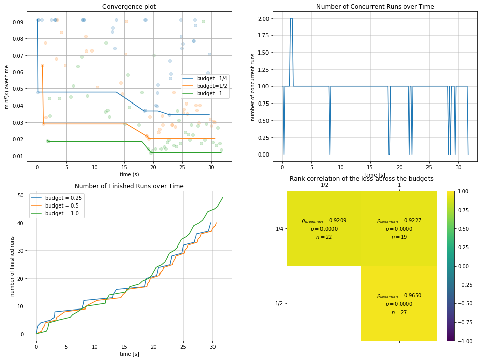
图1的budget分组拟合曲线和图4多budget间相关性图我们在之前已经介绍过了,图2和图3分别阐述了随时间的并行数和随时间的完成情况。
参考文献
